The upcoming interview with David Hendry in the International Journal of Forecasting (now published) sparked a blog post by the Autobox developers on comparing Autobox’s structural change detection to impulse and step-indicator saturation using the isat function in our R-package gets. (Indicator saturation is also available through Autometrics in PcGive/OxMetrics).
We appreciate (and encourage) the comparison, however, indicator saturation was used incorrectly in the author’s example since they do not specify a sensible underlying regression model.
When used correctly, indicator saturation (using isat) detects the hypothesized change with no difficulty. This emphasises that the role of the econometrician/statistician in shaping the analysis using automated procedures remains vital, and must not be neglected. Here we discuss the use of indicator saturation by re-visiting the data example from Autobox to guide future users of isat and our R-package gets.
The data (made available by the authors and also downloadable here) is a time series of T=36 observations with a changepoint (particularly a change in seasonality) around observation t=18. The blog authors apply isat using mostly the default settings of the function.
The default setting (as highlighted in the package manual and discussion paper) of isat are:
- modelling the time series of interest only using a constant (with no other covariates: ar=NULL, mxreg=NULL)
- searching only for step-shift changes in this constant at any point in time (sis=TRUE)
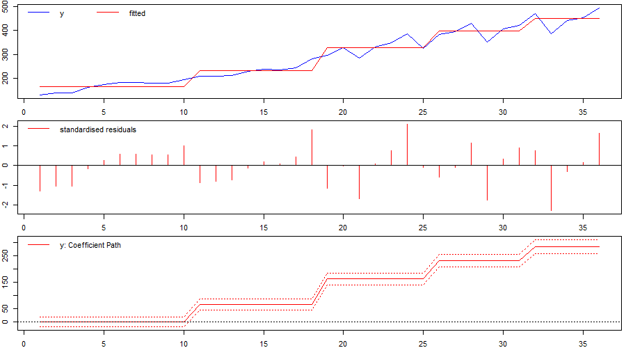
The result – as the authors discover – is that indicator saturation picks up multiple change-points (or shifts) in the intercept and – while the second shift does coincide with the “real” change-point – the other shifts simply approximate the underlying trend of the series which was un-modelled by the authors (reproduced here as Figure 1). Seasonality is also not accounted for because the underlying regression model contains no additional variables. This model-misspecification is apparent when looking at the residual plot or diagnostic tests.
What are the results if we improve the model specification and use indicator saturation?
Let’s consider two cases, first, we assume the time series is trend stationary and contains no autoregressive component:
A) A trend-stationary model
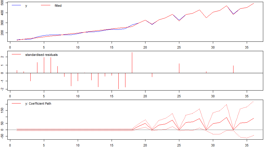
We include a `forced’ linear time-trend in the model specification that is not selected over (mxreg=t), and allow for impulse indicators to pick up outliers and general deviations (iis=TRUE) while, at first, not considering step-shifts (sis=FALSE). We set the significance level to allow for an expected false-positive detection (gauge) of one outlier (t.pval= 1/T). As the results in Figure 2 show, we successfully identify a structural break (or changepoint) in the time series by detecting outliers from observation t=19 onwards. This result also holds when jointly allowing for outliers as well as step-shifts at any point in time (iis=TRUE, sis=TRUE – see replication code below).
Second, let’s estimate a stochastic trend model by considering both first differences and an autoregressive model in levels:
B) A stochastic trend model
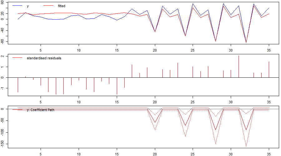
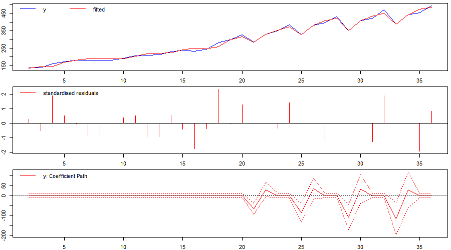
We initially run indicator saturation on first differences of the series including an autoregressive term (ar=1). Again, the problematic period is identified successfully (Figure 3). As impulse indicator saturation (IIS) is valid even in the case of unit-root non-stationary regressors, we also run an AR(1) model of the series in levels. As before, the problematic period is successfully identified (Figure 4).
Beyond the detection of outliers (or simple step-shifts in the intercept), isat in gets is flexible to allow for changes in coefficients on multiple regressors using the user-specified break variable argument (uis). For example, we could allow seasonal patterns to change using designed break functions specified in uis, while also allowing for impulse indicators and step shifts at any point in time. Here we do this by interacting a full set of step-indicators with four seasonal dummy variables and subsequently selecting over this full set of break variables. As above, the problematic period is successfully identified: both through the onset of seasonality (a seasonal indicator significantly enters the model from t=17 onwards reported as “sis17.s4” in the replication code), as well as through additionally detected outlying observations in subsequent periods.
Overall, this comparison highlights the importance of the econometrician/statistician in carefully specifying regression models, and the power and usefulness of indicator saturation methods in detection outliers and structural breaks.
If you would like to try indicator saturation yourself, the R-package gets is freely available and can be downloaded through CRAN or here, there is also an online demonstration using R-studio’s shiny here.
Replication Code:
library(gets)
dat <- read.csv(“gdp.csv”)
plot(dat$gdp, type=”l”)
T <- NROW(dat$gdp) #sample length
t <- as.vector(seq(1:T)) #time trend
y <- as.vector(dat$gdp) #dependent variable
###mis-specified model used by the blog authors
isat(y, t.pval=0.05)
##### A Trend-stationary model with a forced linear time-trend and IIS:
##setting level of significance of selection to one expected false-positive outlier
p_alpha=1/T
##Impulse Indicators only
isat(y, mxreg=t, iis=TRUE, sis=FALSE, t.pval=p_alpha)
##Impulse and Step-Indicators
isat(y, mxreg=t, iis=TRUE, sis=TRUE, t.pval=p_alpha/2)
##### A Stochastic Trend Model
##Using IIS on first differences with an ar(1) regressor
dy <- diff(y, 1)
plot(dy, type=”l”)
isat(dy, ar=1, iis=TRUE, sis=FALSE, t.pval=p_alpha)
###Using IIS on levels with an ar(1) regressor
isat(y, ar=1, iis=TRUE, sis=FALSE, t.pval=p_alpha)
###Extension: Using designed break functions to allow for time-varying seasonality
###creating seasonal dummy variables
library(dummies)
seas_ind <- dummy(dat$seas)
##Creating full set of break functions to select over
s1 <- sim(T)*seas_ind[,1]
s2 <- sim(T)*seas_ind[,2]
s3 <- sim(T)*seas_ind[,3]
s4 <- sim(T)*seas_ind[,4]
S <- cbind(s1, s2, s3, s4)
##setting level of significance of selection to approximately one expected false-positive shift/outlier
p_alpha <- 1/(NCOL(S)+T+(T-1))
seas <- isat(y, mxreg=t, ar=1, uis=S, iis=TRUE, sis=TRUE, plot=FALSE, t.pval=p_alpha)
##print results
seas
###plot results
plot(fitted(seas), type=”l”, col=”red”)
lines(y)